Image Analysis
Chapter describes the ImageN API image analysis operators.
- 9.1 Introduction
- 9.2 Finding the Mean Value of an Image Region
- 9.3 Finding the Extrema of an Image
- 9.4 Histogram Generation
- 9.5 Edge Detection
- 9.6 Statistical Operations
9.1 Introduction
The ImageN API image analysis operators are used to directly or indirectly extract information from an image. The ImageN API supports the following image analysis functions:
- Finding the mean value of an image region
- Finding the minimum and maximum values in an image (extrema)
- Producing a histogram of an image
- Detecting edges in an image
- Performing statistical operations
9.2 Finding the Mean Value of an Image Region
The Mean operation scans a specified region of an image and computes the image-wise mean pixel value for each band within the region. The region of interest does not have to be a rectangle. If no region is specified (null), the entire image is scanned to generate the histogram. The image data pass through the operation unchanged.
The mean operation takes one rendered source image and three parameters:
| Parameter | Type | Description |
|---|---|---|
| roi | ROI | The region of the image to scan. A null value means the whole image. |
| xPeriod | Integer | The horizontal sampling rate. May not be less than 1. |
| yPeriod | Integer | The vertical sampling rate. May not be less than 1. |
The region of interest (ROI) does not have to be a rectangle. It may be null, in which case the entire image is scanned to find the image-wise mean pixel value for each band.
The set of pixels scanned may be reduced by specifying the xPeriod and yPeriod parameters, which define the sampling rate along each axis. These variables may not be less than 1. However, they may be null, in which case the sampling rate is set to 1; that is, every pixel in the ROI is processed.
The image-wise mean pixel value for each band may be retrieved by calling the getProperty method with "mean" as the property name. The return value has type java.lang.Number[#bands].
Listing 9-1 shows a partial code sample of finding the image-wise mean pixel value of an image in the rendered mode.
Listing 9-1 Finding the Mean Value of an Image Region
// Set up the parameter block for the source image and
// the three parameters.
ParameterBlock pb = new ParameterBlock();
pb.addSource(im);   // The source image
pb.add(null);       // null ROI means whole image
pb.add(1);          // check every pixel horizontally
pb.add(1);          // check every pixel vertically

// Perform the mean operation on the source image.
RenderedImage meanImage = JAI.create("mean", pb, null);

// Retrieve and report the mean pixel value.
double[] mean = (double[])meanImage.getProperty("mean");
System.out.println("Band 0 mean = " + mean[0]);
9.3 Finding the Extrema of an Image
The Extrema operation scans a specific region of a rendered image and finds the image-wise minimum and maximum pixel values for each band within that region of the image. The image pixel data values pass through the operation unchanged. The extrema operation can be used to obtain information to compute the scale and offset factors for the amplitude rescaling operation (see Section 7.4, "Amplitude Rescaling").
The region-wise maximum and minimum pixel values may be obtained as properties. Calling the getProperty method on this operation with "extrema" as the property name retrieves both the region-wise maximum and minimum pixel values. Calling it with "maximum" as the property name retrieves the region-wise maximum pixel value, and with "minimum" as the property name retrieves the region-wise minimum pixel value.
The return value for extrema has type double[2][#bands], and those for maximum and minimum have type double[#bands].
The region of interest (ROI) does not have to be a rectangle. It may be null, in which case the entire image is scanned to find the image-wise maximum and minimum pixel values for each band.
The extrema operation takes one rendered source image and three parameters:
| Parameter | Type | Description |
|---|---|---|
| roi | ROI | The region of the image to scan. |
| xPeriod | Integer | The horizontal sampling rate (may not be less than 1). |
| yPeriod | Integer | The vertical sampling rate (may not be less than 1). |
The set of pixels scanned may be further reduced by specifying the xPeriod and yPeriod parameters that represent the sampling rate along each axis. These variables may not be less than 1. However, they may be null, in which case the sampling rate is set to 1; that is, every pixel in the ROI is processed.
Listing 9-2 shows a partial code sample of using the extrema operation to obtain both the image-wise maximum and minimum pixel values of the source image.
**Listing 9-2 Finding the Extrema of an Image*
// Set up the parameter block for the source image and
// the constants
ParameterBlock pb = new ParameterBlock();
pb.addSource(im);   // The source image
pb.add(roi);        // The region of the image to scan
pb.add(50);         // The horizontal sampling rate
pb.add(50);         // The vertical sampling rate

// Perform the extrema operation on the source image
RenderedOp op = JAI.create("extrema", pb);

// Retrieve both the maximum and minimum pixel value
double[][] extrema = (double[][]) op.getProperty("extrema");
9.4 Histogram Generation
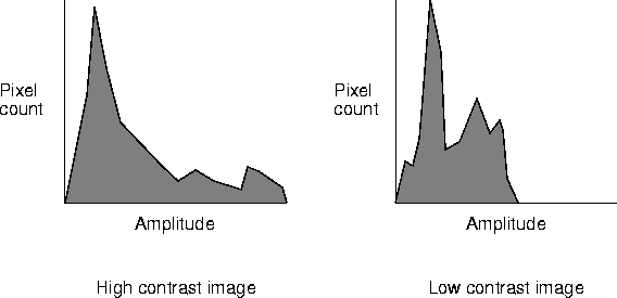
An image histogram is an analytic tool used to measure the amplitude distribution of pixels within an image. For example, a histogram can be used to provide a count of the number of pixels at amplitude 0, the number at amplitude 1, and so on. By analyzing the distribution of pixel amplitudes, you can gain some information about the visual appearance of an image. A high-contrast image contains a wide distribution of pixel counts covering the entire amplitude range. A low contrast image has most of the pixel amplitudes congregated in a relatively narrow range.
Usually, the wider histogram represents a more visually-appealing image.
The primary tasks needed to perform a histogram operation are as follows:
-
Create a
Histogramobject, which specifies the type of histogram to be generated. -
Create a
Histogramoperation with the required parameters or create aParameterBlockwith the parameters and pass it to theHistogramoperation. -
Read the histogram data stored in the object. The data consists of:
- Number of bands in the histogram
- Number of bins for each band of the image
- Lowest value checked for each band
- Highest value checked for each band
9.4.1 Specifying the Histogram
The Histogram object accumulates the histogram information. A histogram counts the number of image samples whose values lie within a given range of values, or "bins." The source image may be of any data type.
The Histogram contains a set of bins for each band of the image. These bins hold the information about gray or color levels. For example, to take the histogram of an eight-bit grayscale image, the Histogram might contain 256 bins. When reading the Histogram, bin 0 will contain the number of 0's in the image, bin 1 will contain the number of 1's, and so on.
The Histogram need not contain a bin for every possible value in the image. It is possible to specify the lowest and highest values that will result in a bin count being incremented. It is also possible to specify fewer bins than the number of levels being checked. In this case, each bin will hold the count for a range of values. For example, for a Histogram with only four bins used with an 8-bit grayscale image, the number of occurrences of values 0 through 63 will be stored in bin 0, occurrences of values 64 through 127 will be stored in bin 1, and so on.
The Histogram object takes three parameters:
| Parameter | Type | Description |
|---|---|---|
| numBins | int[] | Each element specifies the number of bins to be used for one band of the image. The number of elements in the array must match the number of bands in the image. |
| lowValue | float[] | Each element specifies the lowest gray or color level that will be checked for in one band of the image. The number of elements in the array must match the number of bands in the image. |
| highValue | float[] | Each element specifies the highest gray or color level that will be checked for in one band of the image. The number of elements in the array must match the number of bands in the image. |
For an example histogram, see Listing 9-3.
API: org.eclipse.imagen.Histogram
Histogram(int[] numBins, float[] lowValue, float[] highValue)
9.4.2 Performing the Histogram Operation
Once you have created the Histogram object to accumulate the histogram information, you generate the histogram for an image with the histogram operation. The histogram operation scans a specified region of an image and generates a histogram based on the pixel values within that region of the image. The region of interest does not have to be a rectangle. If no region is specified (null), the entire image is scanned to generate the histogram. The image data passes through the operation unchanged.
The histogram operation takes one rendered source image and four parameters:
| Parameter | Type | Description |
|---|---|---|
| specification | Histogram | The specification for the type of histogram to be generated. See Section 9.4.1 |
| roi | ROI | The region of the image to scan. See Section 6.2. |
| xPeriod | Integer | The horizontal sampling rate. May not be less than 1. |
| yPeriod | Integer | The vertical sampling rate. May not be less than 1. |
The set of pixels scanned may be further reduced by specifying the xPeriod and yPeriod parameters that represent the sampling rate along each axis. These variables may not be less than 1. However, they may be null, in which case the sampling rate is set to 1; that is, every pixel in the ROI is processed.
9.4.3 Reading the Histogram Data
The histogram data is stored in the user supplied Histogram object, and may be retrieved by calling the getProperty method on this operation with "histogram" as the property name. The return value will be of type Histogram.
Several get methods allow you to check on the four histogram parameters:
-
The bin data for all bands (
getBins)`` -
The bin data for a specified band (
getBins) -
The number of pixel values found in a given bin for a given band (
getBinSize) -
The lowest pixel value found in a given bin for a given band (
getBinLowValue)
The set of pixels counted in the histogram may be limited by the use of a region of interest (ROI), and by horizontal and vertical subsampling factors. These factors allow the accuracy of the histogram to be traded for speed of computation.
API: org.eclipse.imagen.Histogram
int[][] getBins()int[] getBins(int band)int getBinSize(int band, int bin)float getBinLowValue(int band, int bin)-
void clearHistogram() void countPixels(java.awt.image.Raster pixels, ROI roi, int xStart, int yStart, int xPeriod, int yPeriod)
9.4.4 Histogram Operation Example
Listing 9-3 shows a sample listing for a histogram operation on a three-banded source image.
Listing 9-3 Example Histogram Operation
// Set up the parameters for the Histogram object.
int[] bins = {256, 256, 256};             // The number of bins.
double[] low = {0.0D, 0.0D, 0.0D};        // The low value.
double[] high = {256.0D, 256.0D, 256.0D}; // The high value.

// Construct the Histogram object.
Histogram hist = new Histogram(bins, low, high);

// Create the parameter block.
ParameterBlock pb = new ParameterBlock();
pb.addSource(image);               // Specify the source image
pb.add(hist);                      // Specify the histogram
pb.add(null);                      // No ROI
pb.add(1);                         // Sampling
pb.add(1);                         // periods

// Perform the histogram operation.
dst = (PlanarImage)JAI.create("histogram", pb, null);

// Retrieve the histogram data.
hist = (Histogram) dst.getProperty("histogram");

// Print 3-band histogram.
for (int i=0; i< histogram.getNumBins(); i++) {
   System.out.println(hist.getBinSize(0, i) + " " +
                      hist.getBinSize(1, i) + " " +
                      hist.getBinSize(2, i) + " " +
}
9.5 Edge Detection
Edge detection is useful for locating the boundaries of objects within an image. Any abrupt change in image frequency over a relatively small area within an image is defined as an edge. Image edges usually occur at the boundaries of objects within an image, where the amplitude of the object abruptly changes to the amplitude of the background or another object.
The GradientMagnitude operation is an edge detector that computes the magnitude of the image gradient vector in two orthogonal directions. This operation is used to improve an image by showing the directional information only for those pixels that have a strong magnitude for the brightness gradient.
-
It performs two convolution operations on the source image. One convolution detects edges in one direction, the other convolution detects edges the orthogonal direction. These two convolutions yield two intermediate images.
-
It squares all the pixel values in the two intermediate images, yielding two more intermediate images.
-
It takes the square root of the last two images forming the final image.
The result of the GradientMagnitude operation may be defined as:

where SH(x,y,b) and SV(x,y,b) are the horizontal and vertical gradient images generated from band b of the source image by correlating it with the supplied orthogonal (horizontal and vertical) gradient masks.
The GradientMagnitude operation uses two gradient masks; one for passing over the image in each direction. The GradientMagnitude operation takes one rendered source image and two parameters.
| Parameter | Type | Description |
|---|---|---|
| mask1 | KernelJAI | A gradient mask. |
| mask2 | KernelJAI | A gradient mask orthogonal to the first one. |
The default masks for the GradientMagnitude operation are:
KernelJAI.GRADIENT_MASK_SOBEL_HORIZONTALKernelJAI.GRADIENT_MASK_SOBEL_VERTICAL
These masks, shown in Figure 9-2 perform the Sobel edge enhancement operation. The Sobel operation extracts all of the edges in an image, regardless of the direction. The resulting image appears as an omnidirectional outline of the objects in the original image. Constant brightness regions are highlighted.
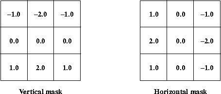
Figure 9-2 Sobel Edge Enhancement Masks
The Roberts' cross edge enhancement operation uses the two masks shown in Figure 9-3. This operation extracts edges in an image by taking the combined differences of directions at right angles to each other to determine the gradient. The resulting image appears as a fairly-coarse directional outline of the objects within the image. Constant brightness regions become black and changing brightness regions become highlighted. The following is a listing of how the two masks are constructed.
float[] roberts_h_data        = { 0.0F,  0.0F, -1.0F,
                                  0.0F,  1.0F,  0.0F,
                                  0.0F,  0.0F,  0.0F
};
float[] roberts_v_data        = {-1.0F,  0.0F,  0.0F,
                                  0.0F,  1.0F,  0.0F,
                                  0.0F,  0.0F,  0.0F
};

KernelJAI kern_h = new KernelJAI(3,3,roberts_h_data);
KernelJAI kern_v = new KernelJAI(3,3,roberts_v_data);
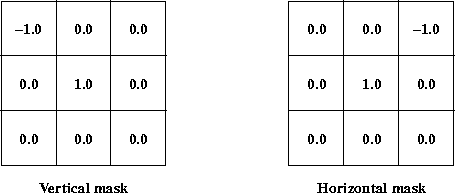
Figure 9-3 Roberts' Cross Edge Enhancement Masks
The Prewitt gradient edge enhancement operation uses the two masks shown in Figure 9-4. This operation extracts the north, northeast, east, southeast, south, southwest, west, or northwest edges in an image. The resulting image appears as a directional outline of the objects within the image. Constant brightness regions become black and changing brightness regions become highlighted. The following is a listing of how the two masks are constructed.
float[] prewitt_h_data        = { 1.0F,  0.0F, -1.0F,
                                  1.0F,  0.0F, -1.0F,
                                  1.0F,  0.0F, -1.0F
};
float[] prewitt_v_data        = {-1.0F, -1.0F, -1.0F,
                                  0.0F,  0.0F,  0.0F,
                                  1.0F,  1.0F,  1.0F
};

KernelJAI kern_h = new KernelJAI(3,3,prewitt_h_data);
KernelJAI kern_v = new KernelJAI(3,3,prewitt_v_data);

Figure 9-4 Prewitt Edge Enhancement Masks
The Frei and Chen edge enhancement operation uses the two masks shown in Figure 9-5. This operation, when compared to the other edge enhancement, operations, is more sensitive to a configuration of relative pixel values independent of the brightness magnitude. The following is a listing of how the two masks are constructed.
float[] freichen_h_data        = { 1.0F,   0.0F,   -1.0F,
                                   1.414F, 0.0F,   -1.414F,
                                   1.0F,   0.0F,   -1.0F
};
float[] freichen_v_data        = {-1.0F,  -1.414F, -1.0F,
                                   0.0F,   0.0F,    0.0F,
                                   1.0F,   1.414F,  1.0F
};

KernelJAI kern_h = new KernelJAI(3,3,freichen_h_data);
KernelJAI kern_v = new KernelJAI(3,3,freichen_v_data);
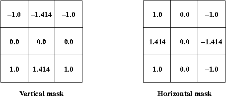
Figure 9-5 Frei and Chen Edge Enhancement Masks
To use a different mask, see Section 6.9, "Constructing a Kernel."
Listing 9-4 shows a sample listing for a GradientMagnitude operation, using the Frei and Chen edge detection kernel.
Listing 9-4 Example GradientMagnitude Operation
// Load the image.
PlanarImage im0 = (PlanarImage)JAI.create("fileload",
                                          filename);

// Create the two kernels.
float data_h[] = new float[] { 1.0F,   0.0F,   -1.0F,
                               1.414F, 0.0F,   -1.414F,
                               1.0F,   0.0F,   -1.0F};
float data_v[] = new float[] {-1.0F,  -1.414F, -1.0F,
                               0.0F,   0.0F,    0.0F,
                               1.0F,   1.414F,  1.0F};

KernelJAI kern_h = new KernelJAI(3,3,data_h);
KernelJAI kern_v = new KernelJAI(3,3,data_v);

// Create the Gradient operation.
PlanarImage im1 =
        (PlanarImage)JAI.create("gradientmagnitude", im0,
                                 kern_h, kern_v);

// Display the image.
imagePanel = new ScrollingImagePanel(im1, 512, 512);
        add(imagePanel);
        pack();
        show();
9.6 Statistical Operations
The StatisticsOpImage class is an abstract class for image operators that compute statistics on a given region of an image and with a given sampling rate. A subclass of StatisticsOpImage simply passes pixels through unchanged from its parent image. However, the desired statistics are available as a property or set of properties on the image (see Chapter 11, "Image Properties").
All instances of StatisticsOpImage make use of a region of interest, specified as an ROI object. Additionally, they may perform spatial subsampling of the region of interest according to xPeriod and yPeriod parameters that may vary from 1 (sample every pixel of the ROI) upwards. This allows the speed and quality of statistics gathering to be traded off against one another.
The accumulateStatistics method is used to accumulate statistics on a specified region into the previously-created statistics object.``
API: org.eclipse.imagen.StatisticsOpImage
StatisticsOpImage()StatisticsOpImage(RenderedImage source, ROI roi, int xStart, int yStart, int xPeriod, int yPeriod, int maxWidth, int maxHeight)