Geometric Image Manipulation

This chapter describes the basics of ImageN's geometric image manipulation functions. The geometric image manipulation operators are all part of the javax.media.operator package.

8.1 Introduction
8.2 Interpolation
8.3 Geometric Transformation
8.4 Perspective Transformation
8.5 Transposing
8.6 Shearing
8.7 Warping

8.1 Introduction

The ImageN geometric image manipulation functions are:

Geometric transformation (Translate, Scale, Rotate, and Affine)
Perspective transformation (PerspectiveTransform)
Transposing (Transpose)
Shearing (Shear)
Warping (Warp, WarpAffine, WarpPerspective, WarpPolynomial, WarpGeneralPolynomial, WarpQuadratic, and WarpOpImage)

Most of these geometric functions require an interpolation argument, so this chapter begins with a discussion of interpolation.

8.2 Interpolation

Several geometric image operations, such as Affine, Rotate, Scale, Shear, Translate, and Warp, use a geometric transformation to compute the coordinate of a source image point for each destination image pixel. In most cases, the destination pixel does not lie at a source pixel location, but rather lands somewhere between neighboring pixels. The estimated value of each pixel is set in a process called interpolation or image resampling.

Resampling is the action of computing a pixel value at a possibly non-integral position of an image. The image defines pixel values at integer lattice points, and it is up to the resampler to produce a reasonable value for positions not falling on the lattice. A number of techniques are used in practice, the most common being the following:

Nearest-neighbor, which simply takes the value of the closest lattice point
Bilinear, which interpolates linearly between the four closest lattice points
Bicubic, which applies a piecewise polynomial function to a 4 x 4 neighborhood of nearby points

The area over which a resampling function needs to be computed is referred to as its support; thus the standard resampling functions have supports of 1, 4, and 16 pixels respectively. Mathematically, the ideal resampling function for a band-limited image (one containing no energy above a given frequency) is the sinc function, equal to sin(x)/x. This has practical limitations, in particular its infinite support, which lead to the use of the standard approximations described above.

In interpolation, each pixel in a destination image is located with integer coordinates at a distinct point D in the image plane. The geometric transform T identifies each destination pixel with a corresponding point S in the source image. Thus, D is the point that T maps to S. In general, S doesn't correspond to a single source pixel; that is, it doesn't have integer coordinates. Therefore, the value assigned to the pixel D must be computed as an interpolated combination of the pixel values closest to S in the source image.

For most geometric transformations, you must specify the interpolation method to be used in calculating destination pixel values. Table 8-1 lists the names used to call the interpolation methods.

Table 8-1 Interpolation Types

Name	Description
INTERP_NEAREST	Nearest-neighbor interpolation. Assigns to point D in the destination image the value of the pixel nearest S in the source image. See Section 8.2.1
INTERP_BILINEAR	Bilinear interpolation. Assigns to Point D in the destination a value that is a bilinear function of the four pixels nearest S in the source image. See Section 8.2.2
INTERP_BICUBIC	Bicubic interpolation. Assigns to point D in the destination image a value that is a bicubic function of the 16 pixels nearest S in the source image. See Section 8.2.3
INTERP_BICUBIC2	Bicubic2 interpolation. Similar to Bicubic, but uses a different polynomial function. See Section 8.2.4

Occasionally, these four options do not provide sufficient quality for a specific operation and a more general form of interpolation is called for. The more general form of interpolation, called table interpolation uses tables to store the interpolation kernels. See Section 8.2.5, "Table Interpolation."

Other interpolation functions may be required to solve problems other than the resampling of band-limited image data. When shrinking an image, it is common to use a function that combines area averaging with resampling to remove undesirable high frequencies as part of the interpolation process. Other application areas may use interpolation functions that operate under other assumptions about image data, such as taking the maximum value of a 2 x 2 neighborhood. The Interpolation class provides a framework in which a variety of interpolation schemes may be expressed.

Many Interpolations are separable, that is, they may be equivalently rewritten as a horizontal interpolation followed by a vertical one (or vice versa). In practice, some precision may be lost by the rounding and truncation that takes place between the passes. The Interpolation class assumes separability and implements all vertical interpolation methods in terms of corresponding horizontal methods, and defines isSeparable to return true. A subclass may override these methods to provide distinct implementations of horizontal and vertical interpolation. Some subclasses may implement the two-dimensional interpolation methods directly, yielding more precise results, while others may implement these using a two-pass approach.

When interpolations that require padding the source such as Bilinear or Bicubic interpolation are specified, the boundary of the source image needs to be extended such that it has the extra pixels needed to compute all the destination pixels. This extension is performed via the BorderExtender class. The type of border extension can be specified as a RenderingHint to the JAI.create method. If no border extension type is provided, a default extension of BorderExtender.BORDER_COPY will be used to perform the extension. See Section 3.7.3, "Rendering Hints."

Listing 8-1 shows a code sample for a rotate operation. First, the type of interpolation is specified (INTERP_NEAREST in this example) using the Interpolation.create method. Next, a parameter block is created and the interpolation method is added to the parameter block, as are all the other parameters required by the operation. Finally, a rotate operation is created with the specified parameter block.

Listing 8-1 Example Using Nearest-neighbor Interpolation

// Specify the interpolation method to be used
interp = Interpolation.create(Interpolation.INTERP_NEAREST);

// Create the parameter block and add the interpolation to it
ParameterBlock pb = new ParameterBlock();
pb.addSource(im);         // The source image
pb.add(0.0F);             // The x origin to rotate about
pb.add(0.0F);             // The y origin to rotate about
pb.add(theta);            // The rotation angle in radians
pb.add(interp);           // The interpolation method

// Create the rotation operation and include the parameter
// block
RenderedOp op JAI.create("rotate", pb, null);

The Interpolation class provides methods for the most common cases of 2 x 1, 1 x 2, 4 x 1, 1 x 4, 2 x 2, and 4 x 4 input grids, some of which are shown in Figure 8-1. These methods are defined in the superclass (Interpolation) to package their arguments into arrays and forward the call to the array versions, to simplify implementation. These methods should be called only on Interpolation objects with the correct width and height. In other words, an implementor of an Interpolation subclass may implement interpolateH(int s0, int s1, int xfrac), assuming that the interpolation width is in fact equal to 2, and does not need to enforce this constraint.

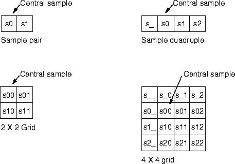
Figure 8-1 Interpolation Samples

Another possible source of inefficiency is the specification of the subsample position. When interpolating integral image data, ImageN uses a fixed-point subsample position specification, that is, a number between 0 and (2n - 1) for some small value of n. The value of n in the horizontal and vertical directions may be obtained by calling the getSubsampleBitsH and getSubsampleBitsV methods. In general, code that makes use of an externally-provided Interpolation object must query that object to determine its desired positional precision.

For float and double images, ImageN uses a float between 0.0F and 1.0F (not including 1.0F) as a positional specifier in the interest of greater accuracy.

API: org.eclipse.imagen.Interpolation

static Interpolation getInstance(int type)
int interpolate(int[][] samples, int xfrac, int yfrac)
float interpolate(float[][] samples, float xfrac, float yfrac)
double interpolate(double[][] samples, float xfrac, float yfrac)
int interpolate(int s00, int s01, int s10, int s11, int xfrac, int yfrac)
float interpolate(float s00, float s01, float s10, float s11, float xfrac, float yfrac)
double interpolate(double s00, double s01, double s10, double s11, float xfrac, float yfrac)
int interpolate(int s__, int s_0, int s_1, int s_2, int s0_, int s00, int s01, int s02, int s1_, int s10, int s11, int s12, int s2_, int s20, int s21, int s22, int xfrac, int yfrac)
float interpolate(float s__, float s_0, float s_1, float s_2, float s0_, float s00, float s01, float s02, float s1_, float s10, float s11, float s12, float s2_, float s20, float s21, float s22, float xfrac, float yfrac)
abstract int getSubsampleBitsH()
int getSubsampleBitsV()

8.2.1 Nearest-neighbor Interpolation

Nearest-neighbor interpolation, also known as zero-order interpolation, is the fastest interpolation method, though it can produce image artifacts called jaggies or aliasing error. Jaggies are image artifacts in which the straight edges of objects appear to be rough or jagged.

Nearest-neighbor interpolation simply assigns to point D in the destination image the value of the pixel nearest S in the source image.

Neighborhoods of sizes 2 x 1, 1 x 2, 2 x 2, 4 x 1, 1 x 4, 4 x 4, N x 1, and 1 x N, that is, all the interpolate() methods defined in the Interpolation class, are supported in the interest of simplifying code that handles a number of types of interpolation. In each case, the central sample is returned and the rest are ignored.

API: org.eclipse.imagen.InterpolationNearest

InterpolationNearest()

8.2.2 Bilinear Interpolation

Bilinear interpolation, also known as first-order interpolation, linearly interpolates pixels along each row of the source image, then interpolates along the columns. Bilinear interpolation assigns to Point D in the destination a value that is a bilinear function of the four pixels nearest S in the source image.

Bilinear interpolation results in an improvement in image quality over nearest-neighbor interpolation, but may still result in less-than-desirable smoothing effects.

Bilinear interpolation requires a neighborhood extending one pixel to the right and below the central sample. If the subsample position is given by (u, v), the resampled pixel value will be:

API: org.eclipse.imagen.InterpolationBilnear

InterpolationBilinear(int subsampleBits)
InterpolationBilinear()

8.2.3 Bicubic Interpolation

Bicubic interpolation reduces resampling artifacts even further by using the 16 nearest neighbors in the interpolation and by using bicubic waveforms rather than the linear waveforms used in bilinear interpolation. Bicubic interpolation preserves the fine detail present in the source image at the expense of the additional time it takes to perform the interpolation.

The bicubic interpolation routine assigns to point D in the destination image a value that is a bicubic function of the 16 pixels nearest S in the source image.

Bicubic interpolation performs interpolation using the following piecewise cubic polynomial:

Bicubic interpolation requires a neighborhood extending one sample to the left of and above the central sample, and two samples to the right of and below the central sample.

API: org.eclipse.imagen.InterpolationBicubic

InterpolationBicubic(int subsampleBits)

8.2.4 Bicubic2 Interpolation

Bicubic2 interpolation is basically the same as bicubic interpolation, but uses a different polynomial function. Bicubic2 interpolation uses the following piecewise cubic polynomial:

Bicubic interpolation requires a neighborhood extending one sample to the left of and above the central sample, and two samples to the right of and below the central sample.

API: org.eclipse.imagen.InterpolationBicubic2

InterpolationBicubic2(int subsampleBits)

8.2.5 Table Interpolation

The previous-described types of interpolation, nearest-neighbor, bilinear, bicubic, and bicubic2, base the interpolation values on a relatively few pixels: one (nearest-neighbor), four (bilinear), or 16 (bicubic and bicubic2). Occasionally, these options don't provide sufficient quality for a specific operation and a general form of interpolation is called for. Table interpolation uses tables to store the interpolation kernels. The set of subpixel positions is broken up into a fixed number of "bins" and a distinct kernel is used for each bin. The number of bins must be a power of two.

An InterpolationTable defines a separable interpolation, with a separate set of kernels for the horizontal and vertical dimensions. The number of bins within each kernel may vary between the two dimensions. The horizontal and vertical kernels may be unique or the same. That is, you can either construct two separate kernels or use the same kernel for both the horizontal and vertical interpolation.

The kernels are stored in both floating- and fixed-point form. The fixed point representation has a user-specified fractional precision. You must specify an appropriate level of precision that will not cause overflow when accumulating the results of a convolution against a set of source pixels, using 32-bit integer arithmetic.

To use table interpolation, create an InterpolationTable with either identical horizontal and vertical resampling kernels or with different horizontal and vertical resampling kernels. The table forms the kernels used for the interpolation.

During a table interpolation operation, the key value of the resampling kernel, generally the center value, is laid over the source image pixel to be processed. The other kernel values lie over neighboring pixels much like a conventional M x N kernel operation. Each source image pixel that is covered by the kernel is then multiplied by the kernel value that lies over it. The multiplication products are then summed together and this sum becomes the pixel value in the destination.

To save memory space and computation time, the table interpolation operation does not use a conventional M x N kernel. Instead, the operation uses separate horizontal and vertical vector arrays (essentially, M x 1 and N x 1) to calculate the same values that a M x N kernel would calculate. The vector arrays allow you to provide fewer data elements for the kernel values. This is particularly significant for large tables with many subsamples.

The basic format for the InterpolationTable constructor is:

     InterpolationTable(int leftPadding, int topPadding, int width,
                        int height, int subsampleBitsH,
                        int subsampleBitsV, int precisionBits,
                        float[] dataH, float[] dataV)

The parameters to the constructor are described in the following paragraphs.

8.2.5.1 Padding

The leftPadding and topPadding parameters define the location of the central sample or key value, relative to the left and top of the horizontal and vertical kernels, respectively. These parameters actually define the number of samples to the left of or above the central sample, as shown in Figure 8-2.

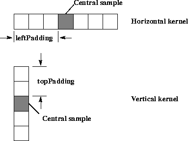
Figure 8-2 Table Interpolation Padding

8.2.5.2 Width and Height

The width and height parameters define the size of the horizontal and vertical kernels, respectively. These parameters specify the number of data elements in each subsample of the kernel. The horizontal and vertical tables can have different kernel sizes. For the two examples shown in Figure 8-2, the width parameter would be 7, the height parameter would be 5.

The getWidth and getHeight methods return the number of samples required for horizontal and vertical resampling, respectively.

8.2.5.3 Subsample Bits

The subsampleBitsH and subsampleBitsV parameters define the number of bins used to describe the horizontal and vertical subpixel positions, respectively. The number of bins must be a power of two, so the values are integers expressed as the log~2~ of the number of horizontal or vertical subsample positions, respectively. The value subsampleBitsH = 1 defines two subsamples per horizontal sample, subsampleBitsH = 2 defines four subsamples per sample, and so on.

For each subsample, you must define separate kernel data. Typically, the kernel values for each subsample are weighted according to the subsample location's proximity to the pixels used in the calculation. The closer a pixel is to the subsample location, the more weight it carries in the kernel.

Figure 8-3 shows how the interpolation tables are used to determine which kernel applies to a particular subsample location. The figure shows a subsample of 4 in both the horizontal and vertical directions.

Typically, the kernel values for each subsample are weighted according to the subsample location's proximity to the pixels used in the calculation. The closer a pixel is to the subsample location, the more weight it carries in the kernel.

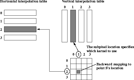
Figure 8-3 Table Interpolation Backwards Mapping

8.2.5.4 Precision

The precisionBits parameter defines the number of fractional bits to be used when resampling integral sample values. The same precision value is used for both horizontal and vertical resampling. It is important to choose an appropriate level of precision that will not cause overflow when accumulating the results of a convolution against a set of source pixels, using 32-bit integer arithmetic.

8.2.5.5 Kernel Data

The kernel data for each table is an array of floating point numbers.
The dataH and dataV parameters specify the floating-point data
values for the horizontal and vertical kernels, respectively. The
number of data elements in the kernel is:: width x 2^subsampleBitsH^ for dataH; height x 2^subsampleBitsV^ for dataV

For a two-element kernel size with eight subsample bins (subsampleBits = 4), you need to define an array of 16 floating point values. The first two values define the kernel for the first subsample, the second two values define the kernel for the second subsample, and so on. For example:

     float[] kernelData = {1.0,    0.0,
                           0.875,  0.125,    // 7/8,  1/8
                           0.75,   0.25,     // 6/8,  2/8
                           0.625,  0.375,    // 5/8,  3/8
                           0.5,    0.5,      // 4/8,  4/8
                           0.375,  0.625,    // 3/8,  5/8
                           0.25,   0.75,     // 2/8,  6/8
                           0.125,  0.875 };  // 1/8,  7/8

The above example creates a bilinear interpolation table with eight subsamples. The kernel values indicate how much influence the source image pixels will have on the destination value. A kernel value of 1 indicates that a source pixel completely determines the value of the destination pixel. A kernel value of 0 indicates that the source pixel has no influence on the destination value.

To preserve the source image's intensity in the destination image, the sum of the data values in each interpolation kernel should equal one. If the kernel values sum to greater than one, the destination image's intensity will be increased. Conversely, if the kernel values sum to less than one, the destination image's intensity will be decreased.

If a value of null is given for dataV, the dataH table data is used for vertical interpolation as well, and the topPadding, height, and subsampleBitsV parameters are ignored.

API: org.eclipse.imagen.InterpolationTable

InterpolationTable(int padding, int width, int subsampleBits, int precisionBits, float[] data)
InterpolationTable(int padding, int width, int subsampleBits, int precisionBits, double[] data)
InterpolationTable(int padding, int width, int subsampleBits, int precisionBits, int[] data)
InterpolationTable(int leftPadding, int topPadding, int width, int height, int subsampleBitsH, int subsampleBitsV, int precisionBits, float[] dataH, float[] dataV)
InterpolationTable(int leftPadding, int topPadding, int width, int height, int subsampleBitsH, int subsampleBitsV, int precisionBits, double[] dataH, double[] dataV)
InterpolationTable(int leftPadding, int topPadding, int width, int height, int subsampleBitsH, int subsampleBitsV, int precisionBits, int[] dataH, int[] dataV)

The InterpolationTable class provides several methods for retrieving an interpolation table's kernel data values, subsample size, and precision.

API: org.eclipse.imagen.InterpolationTable

int getSubsampleBitsH()
int getSubsampleBitsV()
int getPrecisionBits()
int getLeftPadding()
int getTopPadding()
int getWidth()
int getHeight()
int[] getHorizontalTableData()
int[] getVerticalTableData()
float[] getHorizontalTableDataFloat()
float[] getVerticalTableDataFloat()
double[] getHorizontalTableDataDouble()
double[] getVerticalTableDataDouble()

8.3 Geometric Transformation

Geometric transformations provide the ability to reposition pixels within an image. Pixels may be relocated from their (x,y) spatial coordinates in the source image to new coordinates in the destination. Geometric transformations are used, for example, to move (translate), rotate, and scale the geometry of an image. A general type of geometric transformation, warp, is discussed later in this chapter (see Section 8.7, "Warping").

Geometric transformations are used to register multiple images, correct geometric distortions introduced in the image acquisition process, or to add visual effects. The geometric transformation operations discussed here include:

Translation (Translate) - moves an image up, down, left, or right
Scaling (Scale) - enlarges or shrinks an image
Rotation (Rotate) - rotates an image about a given point
Affine (Affine) - includes translation, scaling, and rotation in one operation

All transformation operations are performed by moving pixel values from their original spatial coordinates to new coordinates in the destination image. Every pixel in the source image is passed through this transformation, creating a geometrically-transformed output pixel location. Each pixel of the source image is transformed, pixel by pixel, to its new location in the destination image.

With a very few exceptions, all transformations result in some output pixel locations being missed because no input pixels were transformed there. The missed locations will be devoid of any pixel values and result in a black hole in the destination image. To overcome this problem, intermediate pixel values are estimated through interpolation (See "Interpolation" on page 249). One of four interpolation methods may be selected:

interpolation Methods	Description
INTERP_NEAREST	Use nearest-neighbor interpolation
INTERP_BILINEAR	Use bilinear interpolation
INTERP_BICUBIC	Use bicubic interpolation
INTERP_BICUBIC2	Use bicubic2 interpolation (uses a different polynomial function)

8.3.1 Translation Transformation

Image translation is the spatial shifting of an image up, down, left, or right. The relationships between the source and destination image coordinates are given by the following equation:

: where:

:   *x*~D~ and *y*~D~ are the integer pixel coordinates of the
    destination image
    
:   *t*~x~ and *t*~y~ are the translation values
    
:   *x*\'S and *y*\'S denote the source image point from which the
    pixel estimate is computed.

Translation is often used to register multiple images geometrically. The translation is often carried out to align the images before performing a combination operation, such as image addition, subtraction, division, or compositing.

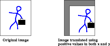
Figure 8-4 Translate Operation

The translate operation takes one rendered or renderable source image and three parameters:

Parameters	Type	Description
xTrans	Float	The displacement in the x direction. The default value is 0.0F.
yTrans	Float	The displacement in the y direction. The default value is 0.0F.
interpolation	Interpolation	The interpolation method for resampling. One of INTERP_NEAREST, INTERP_BILINEAR, INTERP_BICUBIC, or INTERP_BICUBIC2. The default value is null.

The xTrans parameter corresponds to t~x~ and the yTrans parameter corresponds to t~y~ in equation 8.1. If xTrans is positive, the translation is to the right; if negative, to the left. If yTrans is positive, the translation is down; if negative, upward. If both xTrans and yTrans are integral, the operation simply wraps its source image to change the image's position in the coordinate plane.

When interpolations that require padding the source such as bilinear or bicubic interpolation are specified, the boundary of the source image needs to be extended such that it has the extra pixels needed to compute all the destination pixels. This extension is performed via the BorderExtender class. The type of border extension can be specified as a RenderingHint to the JAI.create method. If no border extension type is provided, a default extension of BorderExtender.BORDER_COPY will be used to perform the extension. See Section 3.7.3, "Rendering Hints."

Listing 8-2 shows a code sample for a translate operation using nearest-neighbor interpolation.

Listing 8-2 Example Translate Operation

// Create a ParameterBlock and specify the source and
// parameters.
ParameterBlock pb = new ParameterBlock();
     pb.addSource(im);                   // The source image
     pb.add((float)Math.max(-mx, 0));    // The x translation
     pb.add((float)Math.max(-my, 0));    // The y translation
     pb.add(new InterpolationNearest()); // The interpolation

// Create the translate operation
im = JAI.create("translate", pb, null);

8.3.2 Scaling Transformation

Scaling, also known as minification and magnification, enlarges or shrinks an image. An x-value defines the amount of scaling in the x direction, and a y-value defines the amount of scaling in the y direction. The Scale operation both translates and resizes.

Scaling is often used to geometrically register multiple images prior to performing a combination operation, such as image addition, subtraction, division, or compositing. Scaling can also be used to correct geometric distortions introduced in the image acquisition process, although the Affine operation ("Affine Transformation" on page 272) would be more suitable for this.

For each pixel (x, y) of the destination, the source value at the
fractional subpixel position is constructed by means of an
Interpolation object and written to the destination.

The scale operation takes one rendered or renderable source image and five parameters:

Parameters	Type	Description
xScale	Float	The x scale factor.
yScale	Float	The y scale factor.
xTrans	Float	The x translation.
xTrans	Float	The y translation.
interpolation	Interpolation	The interpolation method for resampling. One of INTERP_NEAREST, INTERP_BILINEAR, INTERP_BICUBIC, or INTERP_BICUBIC2.

When applying scale factors (xScale and yScale) to a source image with width of src_width and height of src_height, the resulting image is defined to have the following dimensions:

         dst_width = src_width * xScale
         dst_height = src_height * yScale

Scale factors greater than 1.0 magnify the image; less than 1.0 minify the image. The xTrans parameter corresponds to t~x~ and the yTrans parameter corresponds to t~y~ in equation 8.1. If xTrans is positive, the translation is to the right; if negative, to the left. If yTrans is positive, the translation is down; if negative, upward.

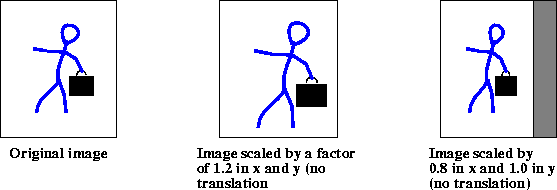
Figure 8-5 Scale Operation

If no Border Extension is specified, the source will not be extended. The scaled image size is still calculated according to the equation specified above. However since there isn't enough source to compute all the destination pixels, only that subset of the destination image's pixels that can be computed will be written in the destination. The rest of the destination will not be written.

Listing 8-3 shows a code sample for a Scale operation using a scale factor of 1.2 and nearest-neighbor interpolation.

Listing 8-3 Example Scale Operation

// Create a ParameterBlock and specify the source and
// parameters
ParameterBlock pb = new ParameterBlock();
     pb.addSource(im);                   // The source image
     pb.add(1.2);                        // The xScale
     pb.add(1.2);                        // The yScale
     pb.add(0.0F);                       // The x translation
     pb.add(0.0F);                       // The y translation
     pb.add(new InterpolationNearest()); // The interpolation

// Create the scale operation
im = JAI.create("scale", pb, null);

8.3.3 Rotation Transformation

The rotate operation rotates an image about a given point by a given angle. Specified x and y values define the coordinate of the source image about which to rotate the image and a rotation angle in radians defines the angle of rotation about the rotation point. If no rotation point is specified, a default of (0,0) is assumed.

A negative rotation value rotates the image counter-clockwise, while a positive rotation value rotates the image clockwise.

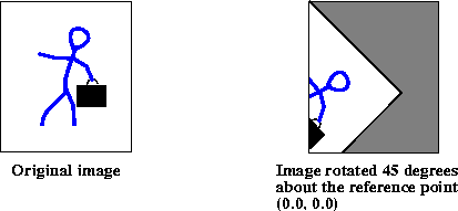
Figure 8-6 Rotate Operation

The rotate operation takes one rendered or renderable source image and four parameters:

Parameters	Type	Description
xOrigin	Float	The x origin to rotate about.
yOrigin	Float	The y origin to rotate about.
angle	Float	The rotation angle in radians.
interpolation	Interpolation	The interpolation method for resampling. One of INTERP_NEAREST, INTERP_BILINEAR, INTERP_BICUBIC, or INTERP_BICUBIC2.

Listing 8-4 shows a code sample for a Rotate operation for a rotation angle of 45 degrees. Since the rotation angle must be specified in radians, the example first converts 45 degrees to radians.

Listing 8-4 Example Rotate Operation

// Create the rotation angle (45 degrees) and convert to
// radians.
int value = 45;
float angle = (float)(value * (Math.PI/180.0F));

// Create a ParameterBlock and specify the source and
// parameters
ParameterBlock pb = new ParameterBlock();
     pb.addSource(im);                   // The source image
     pb.add(0.0F);                       // The x origin
     pb.add(0.0F);                       // The y origin
     pb.add(angle);                      // The rotation angle
     pb.add(new InterpolationNearest()); // The interpolation

// Create the rotate operation
im = JAI.create("Rotate", pb, null);

8.3.4 Affine Transformation

An affine transform is a transformation of an image in which straight lines remain straight and parallel lines remain parallel, but the distance between lines and the angles between lines may change. Affine transformations include translation, scaling, and rotation.

Although there are separate ImageN operations to handle translation, scaling, and rotation, the Affine operation can perform any of these transformations or any combination, such as scale and rotate.

The Affine operation performs (possibly filtered) affine mapping between a source and a destination image. For each pixel (x, y) of the destination, the source value at the fractional subpixel position (x', y') is constructed by means of an Interpolation object and written to the destination.

The affine operation takes one rendered or renderable source image and two parameters:

Parameters	Type	Description
transform	AffineTransform	The affine transform matrix.
interpolation	Interpolation The interpolation method for resampling. One of INTERP_NEAREST, INTERP_BILINEAR, INTERP_BICUBIC, or INTERP_BICUBIC2.

The mapping between the destination pixel (x, y) and the source position (x', y') is given by:

: where m is a 3 x 2 transform matrix that inverts the matrix supplied as the transform argument.

The six elements of the transform matrix are m00, m01, m02, m10, m11, and m12. The constructor looks like this:

     AffineTransform tr = new AffineTransform(m00, m10,
                                              m01, m11,
                                              m02, m12);

These six elements affect the transformation as follows:

Element Description ——————- ————————————————- m00 The x coordinate scale element

m10 The y coordinate shear element

m01 The x coordinate shear element

m11 The y coordinate scale element

m02 The x coordinate translate element

m12 The y coordinate translate element
———————————————————————

The following matrix will translate an image 100 pixels to the right and 200 pixels down:

AffineTransform tr = new AffineTransform(1.0,
                                         0.0,
                                         0.0,
                                         1.0,
                                         100.0,
                                         200.0);

The following matrix will zoom an image by a factor of 2 in both the x and y directions:

AffineTransform tr = new AffineTransform(2.0,
                                         0.0,
                                         0.0,
                                         2.0,
                                         0.0,
                                         0.0);

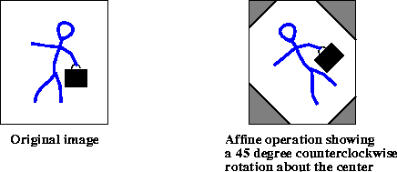
Figure 8-7 Affine Operation

Listing 8-5 shows a code sample for an Affine operation that performs a 45 degree counterclockwise rotation.

Listing 8-5 Example Affine Transform Operation

// Load the image.
String filename = "images/Trees.gif";
PlanarImage im = (PlanarImage)JAI.create("fileload",
                                          filename);

// Create the affine transform matrix.
AffineTransform tr = new AffineTransform(0.707107,
                                        -0.707106,
                                         0.707106,
                                         0.707106,
                                         0.0,
                                         0.0);

// Specify the type of interpolation.
Interpolation interp = new InterpolationNearest();

// Create the affine operation.
PlanarImage im2 = (PlanarImage)JAI.create("affine", im, tr,
                                           interp);

API: `java.awt.geom.AffineTransform

static AffineTransform getTranslateInstance(double tx, double ty)
static AffineTransform getRotateInstance(double theta)
static AffineTransform getRotateInstance(double theta, double x, double y)
static AffineTransform getScaleInstance(double sx, double sy)
static AffineTransform getShearInstance(double shx, double shy)

8.4 Perspective Transformation

Perspective distortions in images are sometimes introduced when the camera is at an angle to the subject. For an example, think of a camera in an aircraft above the earth. If the camera is aimed straight down, the resulting image will be a flat perspective image; that is, no distortion. All objects in the image appear in correct size relative to one another. However, if the camera is angled toward the earth horizon, perspective distortion is introduced. Objects closer to the camera appear larger than same-sized objects farther away from the camera. Perspective distortion has reduced the scale of the objects farthest away.

Perspective distortion can be corrected by applying a perspective transform. The perspective transform maps an arbitrary quadrilateral into another arbitrary quadrilateral, while preserving the straightness of lines. Unlike an affine transformation, the parallelism of lines in the source is not necessarily preserved in the output.

The perspective transform is represented by a 3 x 3 matrix that
transforms homogenous source coordinates (x, y, 1) into
destination coordinates (x', y', w). To convert back into
non-homogenous coordinates, x' and y' are divided by w.

The perspective transform is used with the perspective warp operation. See Section 8.7.7, "Perspective Warp."

API: org.eclipse.imagen.PerspectiveTransform

PerspectiveTransform(float m00, float m01, float m02, float m10, float m11, float m12, float m20, float m21, float m22)
PerspectiveTransform(float[] flatmatrix)
PerspectiveTransform(float[][] matrix)
PerspectiveTransform(double m00, double m01, double m02, double m10, double m11, double m12, double m20, double m21, double m22)
PerspectiveTransform(double[] flatmatrix)
PerspectiveTransform(double[][] matrix)
PerspectiveTransform(AffineTransform transform)

8.4.1 Performing the Transform

The PerspectiveTransform class contains methods that perform the perspective transform on a specified point, an array of point objects, an array of floating point coordinates, or an array of double precision coordinates.

8.4.2 Mapping a Quadrilateral

The PerspectiveTransform class contains methods that may be used to create a perspective transform that can be used to map a unit square to or from an arbitrary quadrilateral and to map an arbitrary quadrilateral onto another arbitrary quadrilateral. The getSquareToQuad methods map the unit square onto an arbitrary quadrilateral:

    (0, 0) → (*x*0, *y*0)\
    (1, 0) → (*x*1, *y*1)\
    (1, 1) → (*x*2, *y*2)\
    (0, 1) → (*x*3, *y*3)

The getQuadToSquare methods map an arbitrary quadrilateral onto the unit square:

    (*x*0, *y*0) → (0, 0)\
    (*x*1, *y*1) → (1, 0)\
    (*x*2, *y*2) → (1, 1)\
    (x3, *y*3) → (0, 1)

The getQuadToQuad methods map an arbitrary quadrilateral onto another arbitrary quadrilateral:

    (*x*0, *y*0) → (*x*0p, *y*0p)\
    (*x*1, *y*1) → (*x*1p, *y*1p)\
    (*x*2, *y*2) → (*x*2p, *y*2p)\
    (*x*3, *y*3) → (*x*3p, *y*3p)

API: org.eclipse.imagen.PerspectiveTransform

static PerspectiveTransform getSquareToQuad(double x0, double y0, double x1, double y1, double x2, double y2, double x3, double y3)
static PerspectiveTransform getSquareToQuad(float x0, float y0, float x1, float y1, float x2, float y2, float x3, float y3)
static PerspectiveTransform getQuadToSquare(double x0, double y0, double x1, double y1, double x2, double y2, double x3, double y3)
static PerspectiveTransform getQuadToSquare(float x0, float y0, float x1, float y1, float x2, float y2, float x3, float y3)
static PerspectiveTransform getQuadToQuad(double x0, double y0, double x1, double y1, double x2, double y2, double x3, double y3, double x0p, double y0p, double x1p, double y1p, double x2p, double y2p, double x3p, double y3p)
static PerspectiveTransform getQuadToQuad(float x0, float y0, float x1, float y1, float x2, float y2, float x3, float y3, float x0p, float y0p, float x1p, float y1p, float x2p, float y2p, float x3p, float y3p)

8.4.3 Mapping Triangles

The PerspectiveTransform class contains methods that may be used to create a perspective transform that can be used to map one arbitrary triangle to another arbitrary triangle. This is done with one of the getTriToTri methods

API: org.eclipse.imagen.PerspectiveTransform

static AffineTransform getTriToTri(double x0, double y0, double x1, double y1, double x2, double y2)
static AffineTransform getTriToTri(float x0, float y0, float x1, float y1, float x2, float y2)

8.4.4 Inverse Perspective Transform

The PerspectiveTransform class contains methods to perform an inverse perspective transform. One of the inverseTransform methods inverse transforms a specified Point2D to another Point2D. Another inverseTransform method inverse transforms an array of double-precision coordinates.

API: org.eclipse.imagen.PerspectiveTransform

Point2D inverseTransform(Point2D ptSrc, Point2D ptDst)
inverseTransform(double[] srcPts, int srcOff, double[] dstPts, int dstOff, int numPts)

8.4.5 Creating the Adjoint of the Current Transform

The PerspectiveTransform class contains a method for creating a new PerspectiveTransform that is the adjoint of the current transform. The adjoint is defined as the matrix of cofactors, which in turn are the determinants of the submatrices defined by removing the row and column of each element from the original matrix in turn.

The adjoint is a scalar multiple of the inverse matrix. Because points to be transformed are converted into homogeneous coordinates, where scalar factors are irrelevant, the adjoint may be used in place of the true inverse. Since it is unnecessary to normalize the adjoint, it is both faster to compute and more numerically stable than the true inverse.

API: org.eclipse.imagen.PerspectiveTransform

public PerspectiveTransform createAdjoint()

8.5 Transposing

The Transpose operation is a combination of flipping and rotating. With a Transpose operation, you can (see Figure 8-8):

Flip an image vertically across an imaginary horizontal axis that runs through the center of the image (FLIP_VERTICAL).
Flip an image horizontally across an imaginary vertical axis that runs through the center of the image (FLIP_HORIZONTAL).
Flip an image across its main diagonal axis, which runs from the upper left to the lower right corner (FLIP_DIAGONAL).
Flip an image across its main anti-diagonal axis, which runs from the upper right to the lower left corner (FLIP_ANTIDIAGONAL).
Rotate an image counterclockwise about its center by 90, 180, or 270 degrees (ROTATE_90, ROTATE_180, ROTATE_270).

The transpose operation takes one rendered or renderable source image and one parameter:

Parameters	Type	Description
type	Integer	The type of flip operation to be performed. One of FLIP_VERTICAL, FLIP_HORIZONTAL, FLIP_DIAGONAL, FLIP_ANTIDIAGONAL, ROTATE_90, ROTATE_180, or ROTATE_270

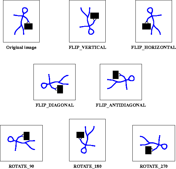
Figure 8-8 Transpose Operations

Listing 8-6 shows sample code for creating a Transpose operation. The example performs a horizontal flip on the source image and creates the destination image im2.

Listing 8-6 Example Transpose Operation

// Create a pattern image.
ParameterBlock pb = new ParameterBlock();
pb.add(image);
PlanarImage im0 = (PlanarImage)JAI.create("awtImage", pb);

// Transpose type : 0=FLIP_VERTICAL
//                : 1=FLIP_HORIZONTAL
//                : 2=FLIP_DIAGONAL
//                : 3=FLIP_ANTIDIAGONAL
//                : 4=ROTATE_90
//                : 5=ROTATE_180
//                : 6=ROTATE_270
int type = 1;

// Create the Transpose operation.
PlanarImage im2 = (PlanarImage)JAI.create("transpose", im0,
                                          type);

8.6 Shearing

Shearing can be visualized by thinking of an image superimposed onto a flexible rubber sheet. If you hold the sides of the sheet and move them up and down in opposite directions, the image will undergo a spatial stretching known as shearing. The shear operation shears an image either horizontally or vertically.

Figure 8-9 Shearing Operations

For each pixel (x, y) of the destination, the source value at the fractional subpixel position (x', y') is constructed by means of an Interpolation object and written to the destination (see "Interpolation" on page 249).

The shear operation takes one rendered source image and five parameters:

Parameters	Type	Description
shear	Float	The shear value.
shearDir	Integer	The shear direction: SHEAR_HORIZONTAL or SHEAR_VERTICAL
xTrans	Float	The x translation.
yTrans	Float	The y translation.
interpolation	Interpolation	The interpolation method for resampling. One of INTERP_NEAREST, INTERP_BILINEAR, INTERP_BICUBIC, or INTERP_BICUBIC2.

For a shearDir parameter of SHEAR_HORIZONTAL:
For a shearDir parameter of SHEAR_VERTICAL:

Listing 8-7 shows a code sample for a Shear operation.

Listing 8-7 Example Shear Operation

// Load the image.
String filename = "images/Picketfence.gif";
PlanarImage im0 = (PlanarImage)JAI.create("fileload",
                                          filename);

imagePanel1 = new ScrollingImagePanel(im0, 512, 512);

// Specify the type of interpolation.
Interpolation interp = new InterpolationNearest();

// Set the shear direction:
//     0 = SHEAR_HORIZONTAL
//     1 = SHEAR_VERTICAL
int shear_dir = 1;

// Set the shear value and the x and y translation values.
float shear_amt = 0.7F;
float x_trans = 50.0F;
float y_trans = 100.0F;

// Create the Shear operation.
PlanarImage im2 = (PlanarImage)JAI.create("shear",
                                           im0,
                                           shear_amt,
                                           shear_dir,
                                           x_trans,
                                           y_trans,
                                           interp);

// Display the image.
imagePanel2 = new ScrollingImagePanel(im2, 512, 512);
add(imagePanel2);
pack();
show();

8.7 Warping

The linear geometric transformations described in Section 8.3, "Geometric Transformation," cannot introduce curvature in the mapping process. Image warping is a type of geometric transformation that introduces curvature into the mapping process. The introduction of curvature is important when an image has been distorted through lens aberrations and other non-linear processes.

Warping transformations, also known as rubber sheet transformations, can arbitrarily stretch the image about defined points. This type of operation provides a nonlinear transformation between source and destination coordinates.

ImageN provides a transformation class, Warp, that is used for non-linear image coordinate transformation. As in the Interpolation class (see Section 8.2, "Interpolation"), pixel positions in the Warp class are represented using fixed-point coordinates, yielding subpixel accuracy but still allowing the use of integer arithmetic. The degree of precision is set by means of the getSubSampleBitsH (horizontal) and getSubSampleBitsV (vertical) parameters to the warpRect method.

The key method of this class is warpRect, which provides the locations of the pixels in source space that map to a given rectangular output region. The output region is specified using normal integer (full pixel) coordinates. The source positions returned by the method are specified in fixed-point, subpixel coordinates.

ImageN supports seven warping functions:

Polynomial warp - a polynomial-based description of an image warp (WarpPolynomial).
General polynomial warp - a general polynomial-based description of an image warp (WarpGeneralPolynomial).
Grid warp - a regular grid-based description of an image warp (WarpGrid).
Quadratic warp - a quadratic-based description of an image warp (WarpQuadratic).
Cubic warp - a cubic-based description of an image warp (WarpCubic).
Perspective warp - a perspective (projective) warp (WarpPerspective).
Affine warp - affine-based warp (WarpAffine).

API: org.eclipse.imagen.Warp

int[] warpRect(int x, int y, int width, int height, int subsampleBitsH, int subsampleBitsV, int[] destRect)
float[] warpRect(int x, int y, int width, int height, float[] destRect)
int[] warpPoint(int x, int y, int subsampleBitsH, int subsampleBitsV, int[] destRect)
float[] warpPoint(int x, int y, float[] destRect)
int[] warpSparseRect(int x, int y, int width, int height, int periodX, int periodY, int subsampleBitsH, int subsampleBitsV, int[] destRect)
abstract float[] warpSparseRect(int x, int y, int width, int height, int periodX, int periodY, float[] destRect)

Rectangle mapDestRect(Rectangle destRect)

8.7.1 Performing a Warp Operation

The Warp operation performs general warping on an image. The warp operation takes one rendered source image and two parameters:

Parameters	Type	Description
warp	Warp	The warp object. One of [WarpAffine]{#WarpAffine} [WarpGrid]{#WarpGrid} [WarpPerspective]{#WarpPerspective} [WarpPolynomial]{#WarpPolynomial} [WarpQuadratic]{#WarpQuadratic} [WarpOpImage]{#WarpOpImage}
interpolation	Interpolation	The interpolation method for resampling. One of INTERP_NEAREST, INTERP_BILINEAR, INTERP_BICUBIC, or INTERP_BICUBIC2.

To create a warp operation:

Create the warp object, which specifies the type of warp operation. The warp object will be one of the following:

Object	Description
WarpAffine	An affine-based image warp. See Affine Waap.
WarpCubic	A cubic-based image warp. See Cubic Warp.
WarpGeneralPolynomial	A polynomial-based image warp for polynomials of a higher degree. See [General Polynomial Warp](#GeneralPolynomialWarp.
WarpGrid	A grid-based image warp where the image may be warped in pieces. See Gridl Warp.
WarpPerspective	A perspective or projective image warp. See Perspective Warp.
WarpPolynomial	A polynomial-based description of an image warp. See Polynomial Warp
WarpQuadratic	A quadratic-based description of an image warp. See [Quadratic Warp)(#QuadraticWarp).

Create the ParameterBlock object and add the source image and the necessary parameters to it. The Warp operation takes two parameters:

Parameters	Description
warp	The Warp object. One of WarpAffine, WarpCubic, WarpGeneralPolynomial, WarpGrid, WarpPerspective, WarpPolynomial, or WarpQuadratic.
interpolation	The interpolation method for resampling. One of INTERP_NEAREST, INTERP_BILINEAR, INTERP_BICUBIC, or INTERP_BICUBIC2.

Create the warp operation with the JAI.create method.

Listing 8-8 shows a sample code for a simple second-order warp operation.

Listing 8-8 Example of a Second-order Warp

// Create WarpPolynomial object for a polynomial warp
// operation.
WarpPolynomial warp;
     float[] coeffs = { 1.0F, 0.0F, 0.0F, 0.0F, 1.0F, 0.0F };

// Create the ParameterBlock and add the parameters to it.
ParameterBlock pb = new ParameterBlock();
     pb.addSource(srcImage);
     pb.add(warp);
     pb.add(new InterpolationNearest());

// Create the warp operation.
dstImage = JAI.create("warp", pb);

8.7.2 Polynomial Warp

The WarpPolynomial class provides a polynomial-based description of an image warp. The mapping is defined by two bivariate polynomial functions X(x, y) and Y(x, y) that define the source x and y positions that map to a given destination (x, y) pixel coordinate.

The functions X(x, y) and Y(x, y) have the form:

The WarpPolynomial constructor takes a coeffs parameter that must
contain a number of coefficients of the form (n + 1)(n + 2) for
some n, where n is the degree power of the polynomial. The
coefficients appear in the following order:

with the coefficients of the polynomial defining the source x coordinates appearing before those defining the y coordinates.

The source (x, y) coordinate is pre-scaled by the factors preScaleX and preScaleY prior to the evaluation of the polynomial. The result of the polynomial evaluations are scaled by postScaleX and postScaleY to produce the destination pixel coordinates. This process allows for better precision of the results.

The number of points needed to control the alignment of the image relates directly to the order of warp. Three control points constitute a first-order warp. Six points constitute a second-order warp. The number of points required for each degree of warp are as follows:

Degree of Warp	Number of Points
1	3
2	6
3	10
4	15
5	21
6	28
7	36

API: org.eclipse.imagen.WarpPolynomial

WarpPolynomial(float[] coeffs)
WarpPolynomial(float[] coeffs, float preScaleX, float preScaleY, float postScaleX, float postScaleY)
float[] getCoeffs()
int getDegree()
static WarpPolynomial createWarp(float[] sourceCoords, int sourceOffset, float[] destCoords, int destOffset, int numCoords, float preScaleX, float preScaleY, float postScaleX, float postScaleY, int degree)

8.7.3 General Polynomial Warp

The WarpGeneralPolynomial class provides a concrete implementation of WarpPolynomial for polynomials of a higher degree.

The mapping is defined by two bivariate polynomial functions X(x, y) and Y(x, y) that define the source X and Y positions that map to a given destination (x, y) pixel coordinate.

The functions X(x, y) and Y(x, y) have the form:

The xCoeffs and yCoeffs parameters must contain the same number of
coefficients of the form (n + 1)(n + 2)/2 for some n, where n
is the non-negative degree power of the polynomial. The coefficients,
in order, are associated with the terms:: 1, x, y, x^2^, x*y, y^2^, ..., x^n^, x^(n -\ 1)^*y, ..., x*y^(n -\ 1)^, y^n^

and coefficients of value 0 can not be omitted.

The destination pixel coordinates (the arguments to the X() and Y() functions) are given in normal integral pixel coordinates, while the output of the functions is given in fixed-point, subpixel coordinates with a number of fractional bits specified by the subsampleBitsH and subsampleBitsV parameters.

API: org.eclipse.imagen.WarpGeneralPolynomial

WarpGeneralPolynomial(float[] xCoeffs, float[] yCoeffs)
WarpGeneralPolynomial(float[] xCoeffs, float[] yCoeffs, float preScaleX, float preScaleY, float postScaleX, float postScaleY)
float[] warpSparseRect(int x, int y, int width, int height, int periodX, int periodY, float[] destRect)

8.7.4 Grid Warp

If polynomial warping is impractical, the image may be warped in pieces using grid warping, also known as control grid interpolation. In the most common implementation of grid warping, specified input control points form a grid of contiguous, horizontally-oriented rectangles in the output image. The mapping from destination pixels to source positions is described by bilinear interpolation between a rectilinear grid of points with known mappings.

Given a destination pixel coordinate (x, y) that lies within a cell having corners at (x0, y0), (x1, y0), (x0, y1), and (x1, y1), with source coordinates defined at each respective corner equal to (sx0, sy0), (sx1, sy1), (sx2, sy2), and (sx3, sy3), the source position (sx, sy) that maps onto (x, y) is given by the following equations:

The source x and y values are interpolated horizontally along the top and bottom edges of the grid cell, and the results are interpolated vertically, as shown in Figure 8-10.

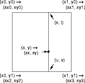
Figure 8-10 Warp Grid

The grid is defined by a set of equal-sized cells starting at (xStart, yStart). The width of each cell is defined by the xStep parameter and the height is defined by the yStep parameter. There are xNumCells cells horizontally and yNumCells cells vertically.

The degree of warping within each cell is defined by the values in the
warpPositions parameter. This parameter must contain the following
values:

These values alternately contain the source x and y coordinates that map to the upper-left corner of each cell in the destination image. The cells are enumerated in row-major order, that is, all the grid points along a row are enumerated first, then the gird points for the next row are enumerated, and so on.

For example, if xNumCells is 2 and yNumCells is 1, the order of the data in the table would be as follows:

     x00, y00, x10, y10, x20, y20, x01, y01, x11, y11, x21, y21

for a total of 2(2 + 1)(1 + 1) = 12 elements.

API: org.eclipse.imagen.WarpGrid

WarpGrid(int xStart, int xStep, int xNumCells, int yStart, int yStep, int yNumCells, float[] warpPositions)
WarpGrid(Warp master, int xStart, int xStep, int xNumCells, int yStart, int yStep, int yNumCells)
float[] warpSparseRect(int x, int y, int width, int height, int periodX, int periodY, float[] destRect)

8.7.5 Quadratic Warp

The WarpQuadratic class provides a quadratic-based description of an image warp. The source position (x', y') of a point (x, y) is given by the following quadratic bivariate polynomial:

API: org.eclipse.imagen.WarpQuadratic

WarpQuadratic(float[] xCoeffs, float[] yCoeffs, float preScaleX, float preScaleY, float postScaleX, float postScaleY)
WarpQuadratic(float[] xCoeffs, float[] yCoeffs)
float[] warpSparseRect(int x, int y, int width, int height, int periodX, int periodY, float[] destRect)

8.7.6 Cubic Warp

The WarpCubic class performs a cubic-based image warp. The source position (x', y') of a point (x, y) is given by the following cubic polynomial:

API: org.eclipse.imagen.WarpCubic

WarpCubic(float[] xCoeffs, float[] yCoeffs, float preScaleX, float preScaleY, float postScaleX, float postScaleY)
WarpCubic(float[] xCoeffs, float[] yCoeffs)
float[] warpSparseRect(int x, int y, int width, int height, int periodX, int periodY, float[] destRect)

8.7.7 Perspective Warp

Perspective distortions in images caused by camera-to-target viewing angle can be restored through perspective warping. Perspective distortion appears as the reduction in scale of an object that recedes from the foreground into the background of the image.

The WarpPerspective class provides a perspective (projective) warp. The transform is specified as a mapping from destination space to source space. In other words, it is the inverse of the normal specification of a perspective image transformation. See Section 8.4, "Perspective Transformation," for a description of the PerspectiveTransform class.

API: org.eclipse.imagen.WarpPerspective

WarpPerspective(PerspectiveTransform transform)
PerspectiveTransform getTransform()
int[] warpSparseRect(int x, int y, int width, int height, int periodX, int periodY, float[] destRect)

8.7.8 Affine Warp

The WarpAffine class provides an affine-based warp. The transform is specified as a mapping from destination space to source space. In other words, it is the inverse of the normal specification of an affine image transformation.

The source position (x', y') of a point (x, y) is given by the quadratic bivariate polynomial:

Listing 8-9 shows a code sample for an affine-based warp operation.

Listing 8-9 Example Affine Warp

// Create the transform parameter (WarpAffine).
double m00 = 0.8;
double m10 = 0.3;
double m01 = -0.7;
double m11 = 1.4;
double m02 = 230.3;
double m12 = -115.7;
AffineTransform transform = new AffineTransform(m00, m10,
                                                m01, m11,
                                                m02, m12);
Warp warp = new WarpAffine(transform);

// Create the interpolation parameter.
Interpolation interp = new InterpolationNearest(8);

// Create the ParameterBlock.
ParameterBlock pb = new ParameterBlock();
pb.addSource(src);
pb.add(warp);
pb.add(interp);

// Create the warp operation.
return (RenderedImage)JAI.create("warp", pb);

API: org.eclipse.imagen.WarpAffine

public WarpAffine(float[] xCoeffs, float[] yCoeffs, float preScaleX, float preScaleY, float postScaleX, float postScaleY)
WarpAffine(float[] xCoeffs, float[] yCoeffs)
public WarpAffine(AffineTransform transform, float preScaleX, float preScaleY, float postScaleX, float postScaleY)
WarpAffine(AffineTransform transform)
AffineTransform getTransform()
float[] warpSparseRect(int x, int y, int width, int height, int periodX, int periodY, float[] destRect)
Rectangle mapDestRect(Rectangle destRect)

Geometric Image Manipulation

8.1 Introduction

8.2 Interpolation

8.2.1 Nearest-neighbor Interpolation

8.2.2 Bilinear Interpolation

8.2.3 Bicubic Interpolation

8.2.4 Bicubic2 Interpolation

8.2.5 Table Interpolation

8.2.5.1 Padding

8.2.5.2 Width and Height

8.2.5.3 Subsample Bits

8.2.5.4 Precision

8.2.5.5 Kernel Data

8.2.5.6 Additional Interpolation Table-related Methods

8.3 Geometric Transformation

8.3.1 Translation Transformation

8.3.2 Scaling Transformation

8.3.3 Rotation Transformation

8.3.4 Affine Transformation

8.4 Perspective Transformation

8.4.1 Performing the Transform

8.4.2 Mapping a Quadrilateral

8.4.3 Mapping Triangles

8.4.4 Inverse Perspective Transform

8.4.5 Creating the Adjoint of the Current Transform

8.5 Transposing

8.6 Shearing

8.7 Warping

8.7.1 Performing a Warp Operation

8.7.2 Polynomial Warp

8.7.3 General Polynomial Warp

8.7.4 Grid Warp

8.7.5 Quadratic Warp

8.7.6 Cubic Warp

8.7.7 Perspective Warp

8.7.8 Affine Warp